Review Which of the following statements about the chi square distribution is false?
Kinh Nghiệm Hướng dẫn Which of the following statements about the chi square distribution is false? 2022
Hoàng T Thu Thủy đang tìm kiếm từ khóa Which of the following statements about the chi square distribution is false? được Cập Nhật vào lúc : 2022-12-19 08:02:05 . Với phương châm chia sẻ Bí kíp Hướng dẫn trong nội dung bài viết một cách Chi Tiết 2022. Nếu sau khi tham khảo nội dung bài viết vẫn ko hiểu thì hoàn toàn có thể lại phản hồi ở cuối bài để Tác giả lý giải và hướng dẫn lại nha.Let X1, X2, …, X10 be a random sample from a standard normal distribution. Find the numbers a and b such that:
Nội dung chính Show- Sampling Properties of Spectral Estimates, Experimental Design, and Spectral ComputationsA9.2 Tables and Graphs for Confidence Intervals, Hypothesis Tests, and Experimental DesignProbability Distributions of Interest8.2.7 Chi-square distributionPlanning AnalysisLarge Sample TestsGoodness of fit tests and categorical data analysis11.5 Tests of independence in contingency tables having fixed marginal totalsComputational Statistics with R4 ResidualsPearson, KarlPearson's Chi-Square TestsWhich of the following is false regarding the given chiWhich of the following statements about chiWhat is not true about the chiWhat is true about the chi
P(a≤∑i=110Xi2≤b)=0.95.
4.2.5.Let X1, X2, …, X5 be a random sample from the normal distribution with mean 55 and variance 223. Let
Y=∑i=15(Xi−55)2/223
andZ=∑i=15(Xi−X¯)2/223.
(a)Find the distribution of the random variables Y and Z.
(b)Are Y and Z independent?
(c)Find (i) P(0.554 ≤ Y ≤ 0.831), and (ii) P(0.297 ≤ Z ≤ 0.484).
4.2.6.Let X and Y be independent chi-square random variables with 14 and 5 degrees of freedom, respectively. Find:
(a)P(|X–Y| ≤ 11.15),
(b)P(|X–Y| ≥ 3.8).
4.2.7.A particular type of vacuum-packed coffee packet contains an average of 16 oz. It has been observed that the number of ounces of coffee in these packets is normally distributed with σ = 1.41 oz. A random sample of 15 of these coffee packets is selected, and the observations are used to calculate s. Find the numbers a and b such that P(a ≤ S2 ≤ b) = 0.90.
4.2.8.An optical firm buys glass slabs to be ground into lenses, and it is known that the variance of the refractive index of the glass slabs is to be no more than 1.04 × 10⁻³. The firm rejects a shipment of glass slabs if the sample variance of 16 pieces selected random exceeds 1.15 × 10⁻³. Assuming that the sample values may be looked on as a random sample from a normal population, what is the probability that a shipment will be rejected even though σ2 = 1.04 × 10⁻³?
4.2.9.Assume that T has a t distribution with 8 degrees of freedom. Find the following probabilities.
(a)P(T ≤ 2.896).
(b)P(T ≤ −1.860).
(c)The value of a such that P(−a < T < a) = 0.99.
4.2.10.Assume that T has a t distribution with 15 degrees of freedom. Find the following probabilities.
(a)P(T ≤ 1.341).
(b)P(T ≥ −2.131).
(c)The value of a such that P(−a < T < a) = 0.95.
4.2.11.A psychologist claims that the mean age which female children start walking is 11.4 months. If 20 randomly selected female children are found to have started walking a mean age of 12 months with standard deviation of 2 months, would you agree with the psychologist's claim? Assume that the sample came from a normal population.
4.2.12.Let U1 and U2 be independent random variables. Suppose that U1 is χ2 with v1 degrees of freedom while U = U1 + U2 is chi-square with v degrees of freedom, where v > v1. Then prove that U2 is a chi-square random variable with v – v1 degrees of freedom.
4.2.13.Show that if X ∼ χ2 (v), then EX = v and Var (X) = 2v.
4.2.14.Let X1, …, Xn be a random sample with Xi ∼ χ2 (1), for i = 1, …, n. Show that the distribution of
Z=X¯−12/n
as n→∞ is standard normal.4.2.15.Find the variance of S2, assuming the sample X1, X2, …, Xn is from N(μ, σ2).
4.2.16.Let X1, X2, …, Xn be a random sample from an exponential distribution with parameter θ. Show that the random variable 2θ−1(∑i=1nXi)∼χ2(2n).
4.2.17.Let X and Y be independent random variables from an exponential distribution with common parameter θ = 1. Show that X/Y has an F distribution. What is the number of the degrees of freedom?
4.2.18.Prove that if X has a t distribution with n degrees of freedom, then X2 ∼ F (1, n).
4.2.19.Let X be F distributed with 9 numerator and 12 denominator degrees of freedom. Find
(a)P(X ≤ 3.87).
(b)P(X ≤ 0.196).
(c)The value of a and b such that P (a < Y < b) = 0.95.
4.2.20.Prove that if X ∼ F(n1,n2), then 1/X ∼ F(n2,n1).
4.2.21.Find the mean and variance of F(n1, n2) random variable.
4.2.22.Let X11,X12,…,X1n1be a random sample with sample mean X¯1from a normal population with mean μ1 and variance σ12, and let X21,X22,…,X2n2be a random sample with sample mean X¯2from a normal population with mean μ2 and variance σ22. Assume the two samples are independent. Show that the sampling distribution of (X¯1−X¯2)is normal with mean μ1–μ2 and variance σ12/n1+σ22/n2.
4.2.23.Let X1, X2, …, Xn1 be a random sample from a normal population with mean μ1 and variance σ2, and Y1, Y2, …, Yn2 be a random sample from an independent normal population with mean μ2 and variance σ2. Show that
T=(X¯−Y¯)−(μ1−μ2)(n1−1)S12+(n2−1)S22n1+n2−2(1n1+1n2)∼T(n1+n2−2).
4.2.24.Show that a t distribution tends to a standard normal distribution as the degrees of freedom tend to infinity.
4.2.25.Show that the mgf of a χ2 random variable with n degrees of freedom is M(t)=(1 – 2t)–n/2. Using the mgf, show that the mean and variance of a chi-square distribution are n and 2n, respectively.
4.2.26.Let the random variables X1, X2, …, X10 be normally distributed with mean 8 and variance 4. Find a number a such that
P(∑i=110(Xi−82)2≤a)=0.95.
4.2.27.Let X2 ∼ F(1,n). Show that X ∼ t(n).
View chapterPurchase book
Read full chapter
URL: https://www.sciencedirect.com/science/article/pii/B978012817815700004X
Sampling Properties of Spectral Estimates, Experimental Design, and Spectral Computations
Lambert H. Koopmans, in The Spectral Analysis of Time Series, 1995
A9.2 Tables and Graphs for Confidence Intervals, Hypothesis Tests, and Experimental Design
List Of Tables And Graphs
Table A9.1. Critical Values of the Chi-Square Distribution.
Table A9.2. Values of log b/a Versus Degrees of Freedom. (Confidence Interval Length for Log Spectral Density.)
Table A9.3. Critical Values of Student's t-Distribution.
Table A9.3. Critical Values of Student's t-Distributiona
kγ.75.90.95.975.99.995.999511.0003.0786.31412.70631.82163.657636.6192.8161.8862.9204.3036.9659.92531.5983.7651.6382.3533.1824.5415.84112.9414.7411.5332.1322.7763.7474.6048.6105.7271.4762 0152.5713.3654.0326.8596.7181.4401.9432.4473.1433.7075.9597.7111.4151.8952.3652.9983.4995.4058.7061.3971.8602.3062.8963.3555.0419.7031.3831.8332.2622.8213.2504.78110.7001.3721.8122.2282.7643.1694.58711.6971.3631.7962.2012.7183.1064.43712.6951.3561.7822.1792.6813.0554.31813.6941.3501.7712.1602.6503.0124.22114.6921.3451.7612.1452.6242.9774.14015.6911.3411.7532.1312.6022.9474.07316.6901.3371.7462.1202.5832.9214.01517.6891.3331.7402.1102.5672.8983.96518.6881.3301.7342.1012.5522.8783.92219.6881.3281.7292.0932.5392.8613.88320.6871.3251.7252.0862.5282.8453.85021.6861.3231.7212.0802.5182.8313.81922.6861.3211.7172.0742.5082.8193.79223.6851.3191.7142.0692.5002.8073.76724.6851.3181.7112.0642.4922.7973.74525.6841.3161.7082.0602.4852.7873.72526.6841.3151.7062.0562.4792.7793.70727.6841.3141.7032.0522.4732.7713.69028.6831.3131.7012.0482.4672.7633.67429.6831.3111.6992.0452.4622.7563.65930.6831.3101.6972.0422.4572.7503.64640.6811.3031.6842.0212.4232.7043.55160.6791.2961.6712.0002.3902.6603.460120.6771.2891.6581.9802.3582.6173.373∞.6741.2821.6451.9602.3262.5763.291
aP(t r.v. with k degrees of freedom ≤ tabled value) = γ. Source: Table abridged from Table III of Fisher, R. A. and Yates, F. (1938). Statistical Tables for Biological, Agricultural, and Medical Research. Oliver & Boyd, Edinburgh, by permission of the authors and publishers.Table A9.4. Critical Values of Fisher's F-Distribution.
Table A9.4. Critical Values of Fisher's F-Distributiona
γl k123456789101215203060120∞.9039.949.553.655.857.258.258.959.459.960.260.761.261.762.362.863.163.3.95161200216225230234237239241242244246248250252253254.97516488008649009229379489579639699779859931000101010101020.994,0505,0005,4005,6205,7605,8605,9305,9806,0206,0606,1106,1606,2106,2606,3106,3406,370.99516,20020,00021,60022,50023,10023,40023,70023,90024,10024,20024,40024,60024,80025,00025,20025,40025,500.908.539.009.169.249.299.339.359.379.389.399.419.429.449.469.479.489.49.9518.519.019.219.219.319.319.419.419.419.419.419.419.519.519.519.519.5.975238.539.039.239.239.339.339.439.439.439.439.439.439.439.539.539.539.5.9998.599.099.299.299.399.399.499.499.499.499.499.499.499.599.599.599.5.995199199199199199199199199199199199199199199199199199.905.545.465.395.345.315.285.275.255.245.235.225.205.185.175.155.145.13.9510.19.559.289.129.018.948.898.858.818.798.748.708.668.628.578.558.53.975317.416.015.415.114.914.714.614.514.514.414.314.314.214.114.013.913.9.9934.130.829.528.728.227.927.727.527.327.227.126.926.726.526.326.226.1.99555.649.847.546.245.444.844.444.143.943.743.443.142.842.542.142.041.8.904.544.324.194.114.054.013.983.953.933.923.903.873.843.823.793.783.76.957.716.946.596.396.266.166.096.046.005.965.915.865.805.755.695.665.63.975412.210.69.989.609.369.209.078.988.908.848.758.668.568.468.368.318.26.9921.218.016.716.015.515.215.014.814.714.514.414.214.013.813.713.613.5.99531.326.324.323.222.522.021.621.421.121.020.720.420.219.919.619.519.3.904.063.783.623.523.453.403.373.343.323.303.273.243.213.173.143.123.11.956.615.795.415.195.054.954.884.824.774.744.684.624.564.504.434.404.37.975510.08.437.767.397.156.986.856.766.686.626.526.436.336.236.126.076.02.9916.313.312.111.411.010.710.510.310.210.19.899.729.559.389.209.119.02.99522.818.316.515.614.914.514.214.013.813.613.413.112.912.712.412.312.1.903.783.463.293.183.113.053.012.982.962.942.902.872.842.802.762.742.72.955.995.144.764.534.394.284.214.154.104.064.003.943.873.813.743.703.67.97568.817.266.606.235.995.825.705.605.525.465.375.275.175.074.964.904.85.9913.710.99.789.158.758.478.268.107.987.877.727.567.407.237.066.976.88.99518.614.512.912.011.511.110.810.610.410.210.09.819.599.369.129.008.88.903.593.263.072.962.882.832.782.752.722.702.672.632.592.562.512.492.47.955.594.744.354.123.973.873.793.733.683.643.573.513.443.383.303.273.23.97578.076.545.895.525.295.124.994.904.824.764.674.574.474.364.254.204.14.9912.29.558.457.857.467.196.996.846.726.626.476.316.165.995.825.745.65.99516.212.410.910.19.529.168.898.688.518.388.187.977.757.537.317.197.08.903.463.112.922.812.732.672.622.592.562.542.502.462.422.382.342.312.29.955.324.464.073.843.693.583.503.443.393.353.283.223.153.083.012.972.93.97587.576.065.425.054.824.654.534.434.364.304.204.104.003.893.783.733.67.9911.38.657.597.016.636.376.186.035.915.815.675.525.365.205.034.954.86.99514.711.09.608.818.307.957.697.507.347.217.016.816.616.406.186.065.95.903.363.012.812.692.612.552.512.472.442.422.382.342.302.252.212.182.18.955.124.263.863.633.483.373.293.233.183.143.073.012.942.862.792.752.71.97597.215.715.084.724.484.324.204.104.033.963.873.773.673.563.453.393.33.9910.68.026.996.426.065.805.615.475.355.265.114.964.814.654.484.404.31.99513.610.18.727.967.477.136.886.696.546.426.236.035.835.625.415.305.19.903.292.922.732.612.522.462.412.382.352.322.282.242.202.152.112.082.06.954.964.103.713.483.333.223.143.073.022.982.912.842.772.702.622.582.54.975106.945.464.834.474.244.073.953.853.783.723.623.523.423.313.203.143.08.9910.07.566.555.995.645.395.205.064.944.854.714.564.414.254.084.003.91.99512.89.438.087.346.876.546.306.125.975.855.665.475.275.074.864.754.64.903.182.812.612.482.392.332.282.242.212.192.152.102.062.011.961.931.90.954.753.893.493.263.113.002.912.852.802.752.692.622.542.472.382.342.30.975126.555.104.474.123.893.733.613.513.443.373.283.183.072.962.852.792.72.999.336.935.955.415.064.824.644.504.394.304.164.013.863.703.543.453.36.99511.88.517.236.526.075.765.525.355.205.094.914.724.534.334.124.013.90.903.072.702.492.362.272.212.162.122.092.062.021.971.921.871.821.791.76.954.543.683.293.062.902.792.712.642.592.542.482.402.332.252.162.112.07.975156.204.774.153.803.583.413.293.203.123.062.962.862.762.642.522.462.40.998.686.365.424.894.564.324.144.003.893.803.673.523.373.213.052.962.87.99510.87.706.485.805.375.074.854.674.544.424.254.073.883.693.483.373.26.902.972.592.382.252.162.092.042.001.961.941.891.841.791.741.681.641.61.954.353.493.102.872.712.602.512.452.392.352.282.202.122.041.951.901.84.975205.874.463.863.513.293.133.012.912.842.772.682.572.462.352.222.162.09.998.105.854.944.434.103.873.703.563.463.373.233.092.942.782.612.522.42.9959.946.995.825.174.764.474.264.093.963.853.683.503.323.122.922.812.69.902.882.492.282.142.051.981.931.881.851.821.771.721.671.611.541.501.46.954.173.322.922.692.532.422.332.272.212.162.092.011.931.841.741.681.62.975305.574.183.593.253.032.872.752.652.572.512.412.312.202.071.941.871.79.997.565.394.514.023.703.473.303.173.072.982.842.702.552.392.212.112.01.9959.186.355.244.624.233.953.743.583.453.343.183.012.822.632.422.302.18.902.792.392.182.041.951.871.821.771.741.711.661.601.541.481.401.351.29.954.003.152.762.532.372.252.172.102.041.991.921.841.751.651.531.471.39.975605.293.933.343.012.792.632.512.412.332.272.172.061.941.821.671.581.48.997.084.984.133.653.343.122.952.822.722.632.502.352.202.031.841.731.60.9958.495.804.734.143.763.493.293.133.012.902.742.572.392.191.961.831.69.902.752.352.131.991.901.821.771.721.681.651.601.541.481.411.321.261.19.953.923.072.682.452.292.182.092.021.961.911.831.751.661.551.431.351.25.9751205.153.803.232.892.672.522.392.302.222.162.051.941.821.691.531.431.31.996.854.793.953.483.172.962.792.662.562.472.342.192.031.861.661.531.38.9958.185.544.503.923.553.283.092.932.812.712.542.372.191.981.751.611.43.902.712.302.081.941.851.771.721.671.631.601.551.491.421.341.241.171.00.953.843.002.602.372.212.102.011.941.881.831.751.671.571.461.321.221.00.975∞5.023.693.122.792.572.412.292.192.112.051.941.831.711.571.391.271.00.996.634.613.783.323.022.802.642.512.412.322.182.041.881.701.471.321.00.9957.885.304.283.723.353.092.902.742.622.522.362.192.001.791.531.361.00
aP(F r.v. with k, I degrees of freedom ≤ tabled value) = γ. Source: Merrington, M., and Thompson, C. M. (1943). “Tables of percentage points of the inverted beta distribution.” Biometrika 33.Table A9.5. Confidence Limits for Multiple Coherence.
Table A9.6. Critical Values for Tests of the Zero Coherence Hypothesis.
Figure A9.1. Graphs of Upper and Lower Confidence Limits for 80% Confidence Intervals for Coherence.
Figure A9.2. Graphs of Upper and Lower Confidence Limits for 90% Confidence Intervals for Coherence.
Figure A9.3. Graphs of the Power Functions of the Zero Coherence Hypothesis Tests, α = 0.05.
Figure A9.4. Graphs of the Power Functions of the Zero Coherence Hypothesis Tests, α = 0.10.
Index to Use of Tables and Graphs in Text
Table A9.1. Pages 274–277
Table A9.2. Page 318
Table A9.3. Pages 285–287
Table A9.4. Pages 284–285, 289–290
Table A9.5. Pages 288–289, 320
Table A9.6. Pages 284, 290, 319–320
Figure A9.1. Pages 283–284, 289, 318–319
Figure A9.2. Pages 283–284, 289, 318–319
Figure A9.3. Pages 284, 290, 319–320
Figure A9.4. Pages 284, 290, 319–320
View chapterPurchase book
Read full chapter
URL: https://www.sciencedirect.com/science/article/pii/B9780124192515500119
Probability Distributions of Interest
N. Balakrishnan, ... M.S Nikulin, in Chi-Squared Goodness of Fit Tests with Applications, 2013
8.2.7 Chi-square distribution
Definition 8.3
We say that a random variableχf2follows the chi-square distribution with f(>0)degrees of freedom if its density is given by
(8.37)qf(x)=12f2Γf2xf2-1e-x/21]0,∞[(x),x∈R1,
whereΓ(a)=∫0∞ta-1e-tdt,a>0,
is the complete gamma function.Let Qf(x)=Pχf2⩽xdenote the distribution function of χf2. It can be easily shown
(8.38)Eχf2=fandVarχf2=2f.
This definition of the chi-square law in not constructive. To construct a random variable χn2,n∈N∗, one may take n independent random variables Z1,…,Zn, following the same standard normal N(0,1)distribution, and then consider the statistic
Z12+⋯+Zn2,forn=1,2,…
It is easily seen that PZ12+⋯+Zn2⩽x=Qn(x), i.e.
(8.39)Z12+⋯+Zn2∼χn2.
Quite often, (8.39) is used for the definition of a chi-square random variable χn2, and here we shall also follow this tradition.
From the central limit theorem, it follows that if n is sufficiently large, then the following normal approximation is valid:
Pχn2-n2n⩽x=Φ(x)+O1n.
This approximation implies the so-called Fisher’s approximation, according to which
P2χn2-2n-1⩽x=Φ(x)+O1n,n→∞.
The best normal approximation of the chi-square distribution is the Wilson–Hilferty approximation given by
Pχn2⩽x=Φxn3-1+29n9n2+O1n,n→∞.
View chapterPurchase book
Read full chapter
URL: https://www.sciencedirect.com/science/article/pii/B9780123971944000089
REGRESSION
Sheldon M. Ross, in Introduction to Probability and Statistics for Engineers and Scientists (Fourth Edition), 2009
REMARKS
A plausibility argument as to why SSR/σ2 might have a chi-square distribution with n −2 degrees of freedom and be independent of A and B runs as follows. Because the Yi are independent normal random variables, it follows that (Yi-E[Yi])/Var(Yi), i =1,…, n are independent standard normals and so
∑i=1n(Yi-E[Yi])2Var(Yi)=∑i=1n(Yi-α-βxi)2σ2~χn2
Now if we substitute the estimators A and B for α and β, then 2 degrees of freedom are lost, and so it is not an altogether surprising result that SSR/σ2has a chi-square distribution with n −2 degrees of freedom.
The fact that SSR is independent of A and B is quite similar to the fundamental result that in normal sampling X¯and S2are independent. Indeed this latter result states that if Y 1,…, Yn is a normal sample with population mean μand variance σ2, then if in the sum of squares ∑i=1n(Yi-μ)2/σ2, which has a chi-square distribution with n degrees of freedom, one substitutes the estimator Y¯for μto obtain the new sum of squares ∑i(Yi-Y¯)2/σ2then this quantity [equal to (n −1)s2/σ2]will be independent of Y¯and will have a chi-square distribution with n −1 degrees of freedom. Since SSR/σ2is obtained by substituting the estimators A and B for α and β in the sum of squares ∑i=1n(Yi-α-βxi)2/σ2, it is not unreasonable to expect that this quantity might be independent of A and B.
When the Yi are normal random variables, the least squares estimators are also the maximum likelihood estimators. To verify this remark, note that the joint density of Y 1,…, Yn is given by
fYi,…,Yn(yi,…,yn)=∏i=1nfYi(yi)=∏i=1n12πσe-(yi-α-βxi)2/2σ2=1(2π)n/2σne-∑i=1n(yi-α-βxi)2/2σ2
Consequently, the maximum likelihood estimators of α and β are precisely the values of α and β that minimize ∑i=1n(yi-α-βXj)2. That is, they are the least squares estimators.
View chapterPurchase book
Read full chapter
URL: https://www.sciencedirect.com/science/article/pii/B978012370483200014X
Planning Analysis
R.H. Riffenburgh, in Statistics in Medicine (Third Edition), 2012
Large Sample Tests
Prior to wide availability of computers and statistical software, several tests were prohibitively manpower intensive when samples were large. “Large sample” methods were developed, particularly for normal, Poisson, signed-rank, and rank-sum tests. These are seldom used today in light of modern computational power. The reader should be aware of their availability.
In addition, the chi-square test of contingency (only; not other uses of the chi-square distribution), developed prior to Fisher’s exact test, is really a large sample alternative that need be used only in cases of multiple categories with large samples.
Exercise 2.5. From Table 2.2, what test on data from DB14 would you choose for the following questions. (a) What will identify or negate age bias? (b) What will identify or negate sex bias? (c) Is eNO from before to after 5 minutes of exercise different between EIB and non-EIB patients?
View chapterPurchase book
Read full chapter
URL: https://www.sciencedirect.com/science/article/pii/B9780123848642000020
Goodness of fit tests and categorical data analysis
Sheldon M. Ross, in Introduction to Probability and Statistics for Engineers and Scientists (Sixth Edition), 2022
11.5 Tests of independence in contingency tables having fixed marginal totals
In Example 11.4.a, we were interested in determining whether gender and political affiliation were dependent in a particular population. To test this hypothesis, we first chose a random sample of people from this population and then noted their characteristics. However, another way in which we could gather data is to fix in advance the numbers of men and women in the sample and then choose random samples of those sizes from the subpopulations of men and women. That is, rather than let the numbers of women and men in the sample be determined by chance, we might decide these numbers in advance. Because doing so would result in fixed specified values for the total numbers of men and women in the sample, the resulting contingency table is often said to have fixed margins (since the totals are given in the margins of the table).
It turns out that even when the data are collected in the manner prescribed above, the same hypothesis test as given in Section 11.4 can still be used to test for the independence of the two characteristics. The test statistic remains
TS=∑i∑j(Nij−eˆij)2eˆij
where
Nij= number of members of sample who have both X-characteristic iundefinedand Y-characteristic jNi= number of members of sample who have X-characteristic iMj= number of members of sample who have Y-characteristic j
and
eˆij=npˆiqˆj=NiMjn
where n is the total size of the sample.
In addition, it is still true that when H0is true, TS will approximately have a chi-square distribution with (r−1)(s−1)degrees of freedom. (The quantities r and s refer, of course, to the numbers of possible values of the X- and Y-characteristic, respectively.) In other words, the test of the independence hypothesis is unaffected by whether the marginal totals of one characteristic are fixed in advance or result from a random sample of the entire population.
Example 11.5.a
A randomly chosen group of 20,000 nonsmokers and one of 10,000 smokers were followed over a 10-year period. The following data relate the numbers of them that developed lung cancer during that period.
SmokersNonsmokersTotalLung cancer621476No lung cancer993819,98629,924Total10,00020,00030,000
Test the hypothesis that smoking and lung cancer are independent. Use the 1 percent level of significance.
Solution
The estimates of the expected number to fall in each ij cell when smoking and lung cancer are independent are
eˆ11=(76)(10,000)30,000=25.33eˆ12=(76)(20,000)30,000=50.67eˆ21=(29,924)(10,000)30,000=9974.67eˆ22=(29,924)(20,000)30,000=19,949.33
Therefore, the value of the test statistic isTS=(62−25.33)225.33+(14−50.67)250.67+(9938−9974.67)29974.67+(19,986−19,949.33)219,949.33=53.09+26.54+.13+.07=79.83
Thus,p-value≈P(χ12>79.83)=1−pchisq(79.83,1)≈0
and so the null hypothesis that whether a randomly chosen person develops lung cancer is independent of whether or not that person is a smoker would be rejected all levels of significance. ■We now show how to use the framework of this section to test the hypothesis that m discrete population distributions are equal. Consider m separate populations, each of whose members takes on one of the values 1,…,n. Suppose that a randomly chosen thành viên of population i will have value j with probability
pi,j,i=1,…,m,j=1,…,n
and consider a test of the null hypothesis
H0:p1,j=p2,j=p3,j=⋯=pm,j,for each j=1,…,n
To obtain a test of this null hypothesis, consider first the superpopulation consisting of all members of each of the m populations. Any thành viên of this superpopulation can be classified according to two characteristics. The first characteristic specifies which of the m populations the thành viên is from, and the second characteristic specifies its value. The hypothesis that the population distributions are equal becomes the hypothesis that, for each value, the proportion of members of each population having that value are the same. But this is exactly the same as saying that the two characteristics of a randomly chosen thành viên of the superpopulation are independent. (That is, the value of a randomly chosen superpopulation thành viên is independent of the population to which this thành viên belongs.)
Therefore, we can test H0by randomly choosing sample members from each population. If we let Midenote the sample size from population i and let Ni,jdenote the number of values from that sample that are equal to j, i=1,…,m, j=1,…,n, then we can test H0by testing for independence in the following contingency table.
ValuePopulationTotals12im1N1,1N2,1…Ni,1…Nm,1N12⋮jN1,jN2,j…Ni,j…Nm,jNj⋮nN1,nN2,n…Ni,nNm,nNnTotalsM1M2…Mi…Mm
Note that Njdenotes the number of sampled members that have value j.
Example 11.5.b
A recent study reported that 500 female office workers were randomly chosen and questioned in each of four different countries. One of the questions related to whether these women often received verbal or sexual abuse on the job. The following data resulted.
CountryNumber Reporting AbuseAustralia28Germany30Japan51United States55
Based on these data, is it plausible that the proportions of female office workers who often feel abused work are the same for these countries?
Solution
Putting the above data in the form of a contingency table gives the following.
CountryTotals1234Receive abuse28305855171Do not receive abuse4724704424451829Totals5005005005002000
We can now test the null hypothesis by testing for independence in the preceding contingency table. R gives that the value of the test statistic and the resulting p-value are
TS=19.51,p-value≈.0002
Therefore, the hypothesis that the percentages of women who feel they are being abused on the job are the same for these countries is rejected the 1 percent level of significance (and, indeed, any significance level above .02 percent). ■View chapterPurchase book
Read full chapter
URL: https://www.sciencedirect.com/science/article/pii/B978012824346600020X
Computational Statistics with R
John Muschelli, ... Ravi Varadhan, in Handbook of Statistics, 2014
4 Residuals
After fitting the model, we can see how well our model predicts the outcome. Residuals are the differences between the observed data and the expected value from the fitted model. By examining how the model predictions depart from the data, we can determine whether the assumptions of the model are being met, identify influential observations, and find ways to improve various aspects of the model.
We will examine a logistic regression model with age, s100b, and NDKA in a logistic regression model from the aSAH dataset (run ?aSAH for definitions):
library(pROC)
data(aSAH)
sah.all <- glm(outcome=="Good"~s100b+age+ndka, data=aSAH, family=binomial)
The working residuals (rWi) are residuals scaled by the variance of the observation, in order to account for the fact that the variance of the response is not independent of the mean:
(2)rWi=yi−E[yi]Var(yi)=yi−niπˆiniπˆi(1−πˆi)
The Pearson residuals (rPi) are standardized by the square root of the variance:
(3)rPi=yi−E[yi]Var(yi)=yi−niπˆiniπˆi(1−πˆi)
As such, these can be considered similar to t-statistics, allowing us to identify observations that fall outside the range predicted by the t-distribution.
Just as the residual sum of squares can be used to indicate goodness of fit in a linear model (LM), the sum of squared Pearson residuals gives an indication of goodness of fit in a GLM, the Pearson's χ2 statistic (χP2).
(4)χP2=∑i=1n(yi−niπˆi)2niπˆi(1−πˆi)
The deviance (D) is another model fit measure based on residuals, based on the log-likelihood of the fitted model. It can be decomposed into the sum of squared deviance residuals, separating the how well the data fit for the yi = 0 versus yi = 1:
(5)D=2∑i=1nyilogyiniπˆi+(ni−yi)logni−yini(1−πˆi)
The sign of the residuals can be obtained by the difference between the observed and fitted values, which indicates if the model over- or underpredicts yi:
(6)rDi=sign(yi−niπˆi)2logyiniπˆi+(ni−yi)logni−yini(1−πˆi)
Under the null hypothesis that the model is correctly specified, the Pearson χ2 and deviance both asymptotically follow a chi-square distribution with N − p degrees of freedom, where N is the number of unique covariate patterns (e.g., if there are 100 people and 2 people have the exact same covariate, then N is 99 since there is a duplicate) and p is the number of parameters estimated. Large values of these statistics relative to the degrees of freedom can indicate poor fit, but failing to reject the null hypothesis does not necessarily indicate adequate model fit. We can then use these to test if the model fit is inadequate:
# Calculate Pearson and Deviance Chi−Square:
1−pchisq(sum(resid(sah.all, type="pearson")ˆ2), sah.all$df.residual)
[1] 0.4931
1−pchisq(sum(resid(sah.all, type="deviance")ˆ2), sah.all$df.residual)
[1] 0.2609
Leverage is a measure of how different an observation is in their covariate pattern irrespective of the outcome. The leverage for the ith observation is given by 1 − hii, where hii is the ith element of the diagonal of the hat matrix H = X(XTX)−1XT. Pearson and deviance residuals can be scaled using the leverage; these scaled residuals have variance 1 and asymptotically have a standard normal distribution if the number of observations corresponding to each pattern of covariates is large enough:
(7)rSi=ri/1−hii
In R, both scaled and unscaled residuals, using resid() and rstandard(), respectively, default to deviance residuals, yet the residuals inside the glm object are actually the working residuals. Externally studentized residuals, residuals obtained from the model leaving out observation i can be obtained using rstudent().
4.1 Interpreting ResidualsIn the aSAH data, since the three covariates are continuous, the conditions for asymptotic normality are unlikely to be met in this dataset. Even if asymptotic normality has not been achieved, comparing the residual distribution to normal or half-normal quantiles can still be used to help detect potential lack of fit. Observations that do not follow a general trend may indicate of lack of fit (Faraway, 2005). We present a quantile–quantile (QQ) plot of the half-normal quantiles compared to the residuals (Fig. 1).
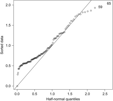
Figure 1. Comparison of the residual distribution to half-normal quantiles.
# Half Normal Plot
library(faraway)
halfnorm(resid(sah.all))
abline(a=0, b=1)
While the residuals do not exactly follow the expected quantiles based on the half-normal distribution, indicated by the diagonal line in Fig. 1, all of the residuals follow a generally contiguous trend. In this dataset, the half-normal residual plot does not indicate any unusual patterns in the residuals.
Just as in ordinary least squares regression, we should also plot the residuals against the fitted values and covariates (Fig. 2).
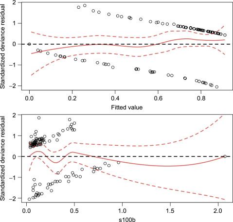
Figure 2. Comparison of fitted values (top) and s100b (bottom) to studentized residuals.
par(mfrow=c(2,1), mar=c(4, 4, 1, 1))
plot(rstandard(sah.all)~fitted(sah.all),
ylab="Standardized Deviance Residual", xlab="Fitted Value")
# Predict LOESS fit over range of fitted values
fit.range <- seq(−.99, .99, 0.01)
rloess <-predict(loess(rstandard(sah.all)~fitted(sah.all)),
newdata=fit.range, se=TRUE)
lines(fit.range, rloess$fit, lwd=2, col=rgb(1,0,0,.75))
lines(fit.range, rloess$fit − qt(0.975, rloess$df)*rloess$se, lty=2, lwd=2, col=rgb(1,0,0,.75))
lines(fit.range, rloess$fit + qt(0.975, rloess$df)*rloess$se, lty=2, lwd=2, col=rgb(1,0,0,.75))
abline(h=0, lty=2, lwd=2)
plot(rstandard(sah.all)~sah.all$model$s100b,
ylab="Standardized Deviance Residual", xlab="s100b")
fit.range <- seq(min(sah.all$model$s100b), max(sah.all$model$s100b), length.out=100)
rloess <-predict(loess(rstandard(sah.all)~aSAH$s100b), newdata=fit.range, se=TRUE)
lines(fit.range, rloess$fit, lwd=2, col=rgb(1,0,0,.75))
lines(fit.range, rloess$fit − qt(0.975, rloess$df)*rloess$se, lty=2, lwd=2, col=rgb(1,0,0,.75))
lines(fit.range, rloess$fit + qt(0.975, rloess$df)*rloess$se, lty=2, lwd=2, col=rgb(1,0,0,.75))
abline(h=0, lty=2, lwd=2)
The LOESS (local regression) (Cleveland et al., 1992) of the residuals on the fitted values is roughly flat, around zero, and smooth with no discernible pattern. If a pattern is observed, the model may be misspecified. Using transformations of the explanatory variables may be needed in that case. We see the LOESS of the residuals on s100b has a discernable pattern within s100b from 0 to 1. This suggests that there may be a nonlinear relationship between s100b and the log-odds of a good functional outcome (Y = 1). We also see one point far away (s100b > 2) from the majority of the s100b data, which may be an influential or outlying point, which we will investigate later using influential point measures. Instead of looking for lack of linearity with the standardized residuals, the correct functional form may be easier to see with partial residuals, which are the residuals from a model without a given covariate in the model (Fig. 3).
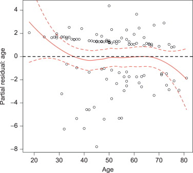
Figure 3. Partial residual plot for age in sah.all logistic regression model.
plot(data.frame(resid(sah.all, type="partial"))$age~sah.all$model$age, ylab="Partial Residual: Age", xlab="Age")
fit.range <- seq(min(sah.all$model$age), max(sah.all$model$age), length.out=100)
rloess <-predict(loess(data.frame(resid(sah.all, type="partial"))$age~aSAH$age), newdata=fit.range, se=TRUE)
lines(fit.range, rloess$fit, lwd=2, col=rgb(1,0,0,.75))
lines(fit.range, rloess$fit − qt(0.975, rloess$df)*rloess$se, lty=2, lwd=2, col=rgb(1,0,0,.75))
lines(fit.range, rloess$fit + qt(0.975, rloess$df)*rloess$se, lty=2, lwd=2, col=rgb(1,0,0,.75))
abline(h=0, lty=2, lwd=2)
4.2 Influential PointsWhile lack of fit can be caused by an improperly specified model, it is also possible that highly influential observations are exerting undue influence over parameter estimates. Influential observations have a large effect on model-based estimation and inference. Outlying observations are ones that are not consistent with general trends observed in the data. An outlier is not always influential, as its removal may not alter the estimates or inference, and an influential point is not always an outlier.
Again, leverage is a measure of how different an observation is in their covariate pattern irrespective of the outcome. The standardized residuals indicate a discrepancy between the model prediction and the observed response. The DFFITS (Belsey et al., 1980) and Cook's distance (Cook, 1977) combine information from the leverage (1 − hii) and the standardized residuals (rDi) to obtain information about which observations may be highly influential:
(8)DFFITSi=rDihii1−hiiDCooki=1phii1−hiirDi2
We can also determine highly influential data points by removing observations one a time, reobtaining the maximum likelihood estimates, and see how and how much they change. This gives the DFBETA (Belsey et al., 1980) statistics for each parameter. Since outliers can also influence the standard errors of parameters, the covariance ratio looks the covariance matrix of the estimated parameters with and without an observation in the dataset.
We can obtain all of these along with indications of whether an observation is influential based on each measure using guidelines proposed by Belsey et al. 1980) and Cook and Weisberg 1980). These guidelines are a function of the number covariates and overall sample size and are implemented on influence.measures.
sah.influence <- influence.measures(sah.all)
# sah.influence$is.inf gives a matrix of logical values for whether a point was
# influential by each measure - can sum by row to find influential points
inf.points <- apply(1*sah.influence$is.inf, 1, sum)
inf.points <- inf.points[which(inf.points > 0)]
# Find which influence measures were notable, and print their values
sah.influence$is.inf[which(rownames(sah.influence$infmat) %in%names(inf.points)),]
dfb.1_dfb.s100dfb.agedfb.ndkadffitcov.rcook.dhat48FALSEFALSEFALSEFALSEFALSETRUEFALSEFALSE57FALSEFALSEFALSEFALSETRUETRUEFALSETRUE90FALSEFALSEFALSEFALSEFALSETRUEFALSETRUE97FALSEFALSEFALSEFALSEFALSETRUEFALSEFALSE101FALSEFALSEFALSEFALSEFALSETRUEFALSETRUE
sah.influence$infmat[which(rownames(sah.influence$infmat) %in%names(inf.points)),]
dfb.1_dfb.s100dfb.agedfb.ndkadffitcov.rcook.dhat480.07577−0.08465−0.007937−0.22042−0.23711.1150.0088330.0891557−0.365340.060700.1613580.895640.93551.1710.2462510.21264900.09693−0.01882−0.1653040.290040.36841.1670.0225560.1383997−0.04776−0.180760.100803−0.01528−0.20971.1110.0067680.082931010.161500.00633−0.059282−0.50549−0.53601.2450.0501980.20108
In the presence of influential points, it may be wise to conduct a sensitivity analysis, using robust estimates of the regression coefficients, obtained using robust/resistant estimation techniques (Cantoni, 2004; Cantoni and Ronchetti, 2001, 2006; Heritier et al., 2009; Valdora and Yohai, 2014; Wang et al., 2014). These estimates are less prone to bias from influential data.
library(robust)
sah.all.rob <- glmrob(outcome=="Good"~s100b+age+ndka, data=aSAH, family=binomial)
summary(sah.all)$coefficients
EstimateStd. Errorz valuePr(>|z|)(Intercept)3.458580.995443.4745.120e−04s100b−5.046621.25878−4.0096.094e−05age−0.022020.01693−1.3011.934e−01ndka−0.031310.01631−1.9205.484e−02
summary(sah.all.rob)$coefficients
EstimateStd. Errorz valuePr(>|z|)(Intercept)3.539621.024183.4560.0005482s100b4.744781.26221−3.7590.0001705age−0.024570.01729−1.4210.1552039ndka−0.031570.01650−1.9130.0557637
Since the differences in parameters are small relative to their standard errors, and the standard errors are consistent between models, it looks like the influential points are not unduly influential.
View chapterPurchase book
Read full chapter
URL: https://www.sciencedirect.com/science/article/pii/B9780444634313000073
Pearson, Karl
M. Eileen Magnello, in Encyclopedia of Social Measurement, 2005
Pearson's Chi-Square Tests
At the turn of the century, Pearson reached a fundamental breakthrough in his development of a modern theory of statistics when he found the exact chi-square distribution from the family of gamma distributions and devised the chi-square (χ2, P) goodness-of-fit test. The test was constructed to compare observed frequencies in an empirical distribution with expected frequencies in a theoretical distribution to determine “whether a reasonable graduation had been achieved” (i.e., one with an acceptable probability). This landmark achievement was the outcome of the previous 8 years of curve fitting for asymmetrical distributions and, in particular, of Pearson's attempts to find an empirical measure of a goodness-of-fit test for asymmetrical curves.
Four years later, he extended this to the analysis of manifold contingency tables and introduced the “mean square contingency coefficient,” which he also termed the chi-square test of independence (which R. A. Fisher termed the chi-square statistic in 1923). Although Pearson used n − 1 for his degrees of freedom for the chi-square goodness-of-fit test, Fisher claimed in 1924 that Pearson also used the same degrees of freedom for his chi-square test of independence. However, in 1913 Pearson introduced what he termed a “correction” (rather than degrees of freedom) for his chi-square test of independence of 1904. Thus, he wrote, if x = number of rows and λ = number of columns, then on average the correction for the number of cells is (x − 1) (λ − 1)/N. [As may be seen, Fisher's degrees of freedom for the chi-square statistic as (r − 1) (c − 1) is very similar to that used by Pearson in 1913.]
Pearson's conception of contingency led once to the generalization of the notion of the association of two attributes developed by his former student, G. Udny Yule. Individuals could now be classed into more than two alternate groups or into many groups with exclusive attributes. The contingency coefficient and the chi-square test of independence could then be used to determine the extent to which two such systems were contingent or noncontingent. This was accomplished by using a generalized theory of association along with the mathematical theory of independent probability.
Which of the following is false regarding the given chi
Answer and Explanation: Option (A) is a false statement because of the reason that if the degrees of freedom increase then the chi-square distribution gets close to a normal distribution which is symmetric around the mean.Which of the following statements about chi
The statement that the chi-square distribution is symmetrical just like the normal distribution is incorrect. The chi-square distribution is not symmetrical; it is skewed. All other statements are correct.What is not true about the chi
Which statement is NOT correct about the chi-square test statistic? A value close to 0 would indicate expected counts are much different from observed counts. A large value of the test statistic would be in support of the alternative hypothesis.What is true about the chi
A chi-square distribution is a continuous probability distribution. The shape of a chi-square distribution depends on its degrees of freedom, k. The mean of a chi-square distribution is equal to its degrees of freedom (k) and the variance is 2k. The range is 0 to ∞. Tải thêm tài liệu liên quan đến nội dung bài viết Which of the following statements about the chi square distribution is false?
Post a Comment